Build a DL Library from Scratch (Part1) - Background

titaneric published on January 05, 2021

8 min, 1491 words

Categories: Notes

Introduction

This is an article to elaborate on the detail of how I build my personal project Autodiff from scratch. It may take several parts to finish, including the fundamental backpropagation, computational graph, auto differentiation concept, implementation detail, brief prior frameworks implementation detail, demonstration results, testing, and finally, what I learn during the process. Please be patient and I promised I'll finish the series this year (2021).

Disclaimer

I am not a native speaker and I do not consider myself a deep learning expert, these series act more like personal notes rather than lessons. However, I'll be glad to hear someone point out my grammar issue and give their professional insight. These series are the extension of my Final presentation, please take a look if you don't have much time to read the whole series.

Motivation

First, let's talk about the reason why I wrote this project. In my learning experience of deep learning, I observed that a few online lessons and books just listed the APIs that the framework provided e.g., CNN, RNN, the Transformer, etc. However, the API may be deprecated, the discovery in this domain remain continuously changed. Equipped with something unchanged including the fundamental knowledge is more important than knowing how to call a 3-Linear Layers in PyTorch.

Of course, some great lessons talk about the math behind network design, its architecture, and application. They are kindly shared freely on the Internet, and lots of audiences are impressed and highly educated (including me). Be aware of this knowledge help the learner level up their ability. However, I want to get my hand dirty and build my unique library, so that's the reason why I start this project.

Nevertheless, starting everything from scratch is hard for me. I need an existed project to teach me which are the necessary steps so I could digest and simplify them. I was lucky to find one of the lessons taught at the University of Toronto which introduced a concept called automatic differentiation and its implementation i.e., Autograd. I was fascinated and took lots of time to learn from the various lesson and trace some source code. After that, I create my unique deep learning library which is simple enough to tackle the real-world problem.

Background

It's too wordy to talk about my motivation. Let's begin our journey to introduce some concepts. We'll introduce the computational graph and the backpropagation algorithm in this post. In these series, I assume the reader may have basic knowledge of Calculus, some deep learning background, or at least, the eagerness to learn something new.

Computational Graph

We all know the graph in data structure created by nodes and edges. In Computer Science, we could solve many graph problems explicitly (e.g., Traveling Salesman Problem, single-source shortest path, etc.) or implicitly (by reduction, e.g., SAT problem); In Deep Learning, the computation could also be represented by the graph, i.e., the node indicates the operands (input) and the edge indicates the operator (computation). For example, given a simple formula \((3 - 2) + 1\), the corresponding graph is

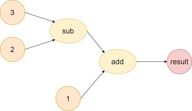
Note that the order of arguments matters. The correct order induces the right result and could receive the correct response (backpropagation) even in the order-invariant calculation (e.g., add and multiply operation).

It's easy to understand the concept by simply glance the computational graph. Besides, the calculation could be in any number of operands, operators, or even high-level modules. For instance, a linear layer may consist of many nodes, layers, and pairs of connections (may not be a complete bipartite graph and could contain self-loop), or even a monster -- the Transformer formed with different modules and layers of encoder or decoder. There is an old saying, a picture is worth of thousand words. It's recommended to sketch the complicated concept, you will gain a lot during the drawing process and explain it to your coworker.

Backpropagation algorithm

The core of deep learning is the backpropagation algorithm. In the computational graph session, we build the graph by a forward pass, i.e., evaluating the computation. On the other hand, we could calculate the gradient of the given calculation by backpropagation.

We could use the last example, \((3 - 2) + 1\) to illustrate and transform them into algebraic way \(z = (a - b) + c\). Suppose we want to compute the gradient of \(z\) w.r.t. \(c\). It's easy to get it directly. \[\frac{\partial z}{\partial c}=\frac{\partial[(a-b) + c]}{\partial c} = 0 + 1 = 1\] \((a-b)\) could be seemed as an constant to \(c\), so we get zero; On the other hand, the derivative of variable \(c\) w.r.t. \(c\) is \(1\).

Next, we try to take the derivative of z w.r.t. b by the chain rule. We could use the following procedure to compute the result.

Let \(d = (a - b)\), so we let \(z = d + c\). \[ \begin{aligned} \frac{\partial[(a-b) + c]}{\partial b} &=\frac{\partial d+c}{\partial d}\cdot \frac{\partial d}{\partial b}\\ &=1\cdot \frac{\partial a-b}{\partial b}\\ &=1\cdot -1\\ &= -1 \end{aligned} \]

We could use the chain rule to easily calculate the complicated derivative w.r.t. any variable. It seems easy to take the derivatives of the above equation without chain rule, but what about a slightly difficult equation called the sigmoid function?

\[y = \frac{1}{1 + e^{-z}}\]

If we want to get the derivative of above equation w.r.t. \(z\), the interesting way to compute is

Let \(a = 1 + e^{-z}\), \[ \begin{aligned} \frac{\partial y}{\partial z} &= \frac{\partial \frac{1}{a}}{\partial z}\\ &= \frac{\partial ({\color{red}{{a}^{-1}}})}{\partial a} \cdot \frac{\partial a}{\partial z}\\ &= -1 {a}^{-2} \cdot \frac{\partial a}{\partial z}\\ &= -1 {(1 + e^{-z})}^{-2} \cdot \frac{\partial (1 + e^{-z})}{\partial z}\\ \end{aligned} \] Let \(b = e^{-z}\), \[ \begin{aligned} \frac{\partial y}{\partial z} &= -1 {(1 + e^{-z})}^{-2} \cdot \frac{\partial (1 + e^{-z})}{\partial z}\\ &= -1 {(1 + e^{-z})}^{-2} \cdot \frac{\partial ({\color{red}{1 + b}})}{\partial b}\cdot \frac{\partial (b)}{\partial z}\\ &= -1 {(1 + e^{-z})}^{-2} \cdot 1 \cdot \frac{\partial (e^{-z})}{\partial z}\\ \end{aligned} \] Let \(c = -z\), \[ \begin{aligned} \frac{\partial y}{\partial z} &= -1 {(1 + e^{-z})}^{-2} \cdot 1 \cdot \frac{\partial (e^{-z})}{\partial z}\\ &= -1 {(1 + e^{-z})}^{-2} \cdot 1 \cdot \frac{\partial ({\color{red}{e^{c}}})}{\partial c} \cdot \frac{\partial (c)}{\partial z}\\ &= -1 {(1 + e^{-z})}^{-2} \cdot 1 \cdot e^{c} \cdot \frac{\partial (c)}{\partial z}\\ &= -1 {(1 + e^{-z})}^{-2} \cdot 1 \cdot e^{-z} \cdot \frac{\partial (-z)}{\partial z}\\ \end{aligned} \] Let \(d = z\) \[ \begin{aligned} \frac{\partial y}{\partial z} &= -1 {(1 + e^{-z})}^{-2} \cdot 1 \cdot e^{-z} \cdot \frac{\partial (-z)}{\partial z}\\ &= -1 {(1 + e^{-z})}^{-2} \cdot 1 \cdot e^{-z} \cdot \frac{\partial ({\color{red}{-d}})}{\partial d} \cdot \frac{\partial (d)}{\partial z}\\ &= -1 {(1 + e^{-z})}^{-2} \cdot 1 \cdot e^{-z} \cdot -1 \cdot \frac{\partial (z)}{\partial z}\\ &= -1 {(1 + e^{-z})}^{-2} \cdot 1 \cdot e^{-z} \cdot -1 \cdot 1\\ \end{aligned} \]

Notice that some operation are replaced by fundamental operation colored with red like reciprocal (\(a^{-1}\)), exponential (\(e^{c}\)), negative (\(-d\)), and add operation (\(1+b\)).

In this way, we could systematically calculate the derivative of the given formula only known for the corresponding derivative of fundamental operation and chain rule. In other words, we could write a program to compute the derivative in a systematic manner. Besides, we don't have to make a program to learn extra knowledge like sum, product, and quotient rules, since the program has already been educated for add, multiplication, and division operation, respectively.

Let's combine this with the computational graph below

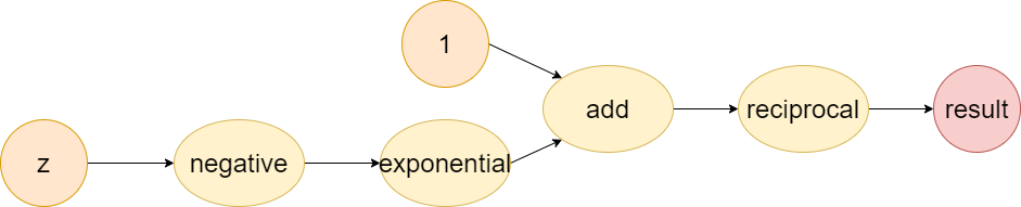
The figure shows that the forward-pass builds the graph from the variables, to some basic operation and finally to the results, but we compute the gradient backwardly from the result to the last, the second last, and to the first basic operation.

Conclusion

We could conclude today's content with the following

The computational graph could be any form, from the basic operation in math to the more complicated one like layers, modules, and models.
The forward pass builds the computational graph, the backward pass computes the gradient with respect to some variable.

Hope that the readers could understand today's concept because, in the next part, we will introduce the auto differentiation by these two ideas. (Spoiled alert: gradient calculation in Backpropagation session)

Thank you for reading and please be patient with the next part.