Build a DL Library from Scratch (Part2) - Backpropagation

Introduction

Previously, I talked about my motivation and introduced some background including the computational graph and backpropagation algorithm. Let's move on to learn something new!

Background

Auto-Differentiation

Equipped with chain rule and fundamental derivative, we could calculate the gradient of given function w.r.t. any variable by auto-differentiation.

We may refresh our memory by reviewing the previous example again. Before that, we should introduce some terms used in this post.

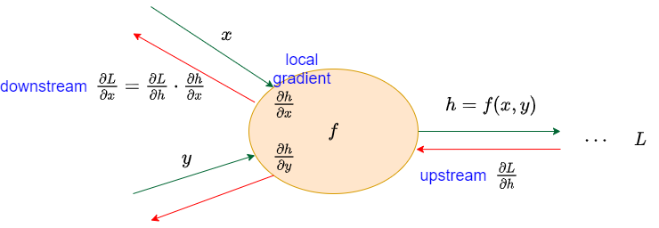
Given a function \(h = f(x,y)\), we know that \(x\) and \(y\) is the input for function \(f\), and the \(h\) is the result. This is the forward pass.

When calculating the gradient of this function, we need backpropagation. Suppose that the loss \(L\) is the final result and the \(\frac{\partial{L}}{\partial{h}}\) is already calculated in the last node which is also called upstream.

We may derive the gradient of function \(f\) w.r.t. input \(x\). Cause function \(f\) is the fundamental operation like multiplication, add or exponential. We could easily receive the derivative result \(\frac{\partial{h}}{\partial{x}}\) called local gradient.

Finally, we have \(\frac{\partial{L}}{\partial{x}}\) called downstream by chain rule \(\frac{\partial{L}}{\partial{x}}=\frac{\partial{L}}{\partial{h}}\cdot\frac{\partial{h}}{\partial{x}}\). Downstream is the upstream to the next node, gradient is similar to water flow passing through each operation nodes to the derivative target.

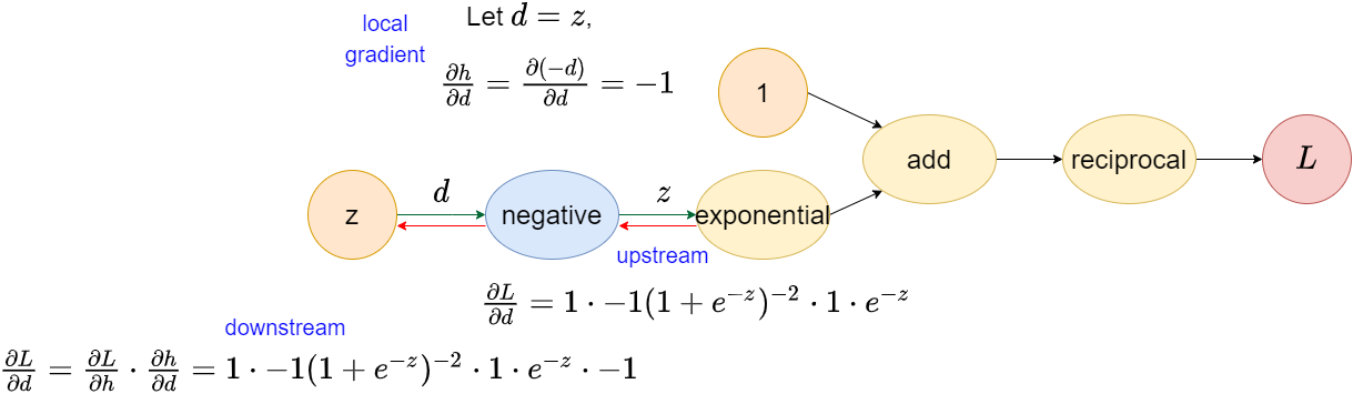
We may re-visit the last example to illustrate the autodiff. We will step by step (or node by node) to derive the result.

Given a sigmoid function, We want to get the derivative of function \(y\) w.r.t. \(z\). \[y = \frac{1}{1 + e^{-z}}\]

Reciprocal operator

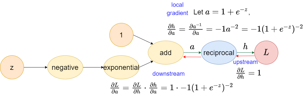
⚠ Notice that upstream here is constant 1 for outermost operation (the closest one to output) in the computational graph. In fact, it is not 1, it is the tensor filled with scalar 1 which shape is equal to the output.

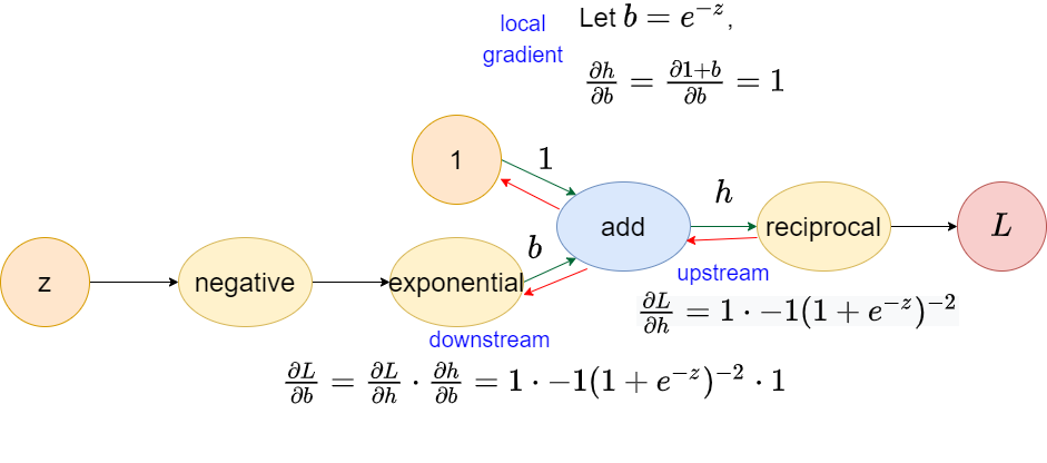
Add operator

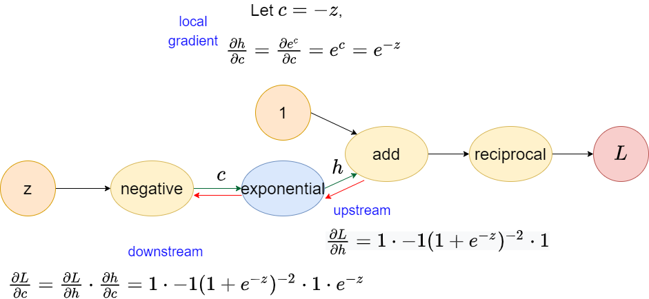
Exponential operator

Negative operator

Validation

Downstream \(\frac{\partial{L}}{\partial{z}}=\frac{\partial{L}}{\partial{d}}=1 \cdot -1(1+e^{-z})^{-2}\cdot 1 \cdot e^{-z} \cdot -1\) is the final result we want. We could validate the result by numerical way that we learned in the Calculas class, which is \[f'(x) = \lim_{\epsilon\to 0} \frac{f(x + \epsilon) - f(x)}{\epsilon}\]

⚠ Notice that this validation could validate almost any function which could be used in the unit test. This could be found in various deep learning frameworks.

We could feed \(z=0\) and \(\epsilon=0.01\) to original function \(f(z)=\frac{1}{1+e^{-z}}\). \[f(0)=\frac{1}{1+1}=\frac{1}{2}=0.5\] \[f(0+0.01)=\frac{1}{1+e^{-0.01}}\approx\frac{1}{1+0.99}\approx 0.5025\] \[f'(0)=\frac{f(0+0.01)-f(0)}{0.01}\approx\frac{0.5025-0.5}{0.01}=0.25\]

Next, we feed \(z=0\) to \(\frac{\partial{L}}{\partial{z}}\) that we computed earlier, \[\frac{\partial{L}}{\partial{z}}\Bigr|_{\substack{z=0}}=1 \cdot -1(1+e^{0})^{-2}\cdot 1 \cdot e^{0} \cdot -1=1 \cdot -1(2)^{-2} \cdot 1 \cdot -1 = 0.25\] We find that both result is identical, which means that our auto-differentiation is correct!

We almost finish, but what if the operation has multiple upstreams? We need the multivariate chain rule.

Multivariate chain rule

Consider a function \(f\), which is composed by another two function \(g(x)\) and \(h(x)\), corresponding \(f'(x)\) is \[\frac{\partial{f}}{\partial{x}}=\frac{\partial{f}}{\partial{h}}\cdot\frac{\partial{h}}{\partial{x}}+\frac{\partial{f}}{\partial{g}}\cdot\frac{\partial{g}}{\partial{x}}\]

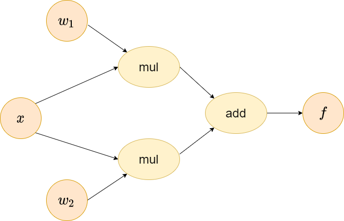
Again, give a tiny example which is commonly seen in the neural networks, a subset of linear layer \(f(x)=g(x)+h(x)\) where \(h(x)=w_1x\) and \(g(x)=w_2x\). The computational graph of this function is similar to the following. We could see that x has two upstreams, which could leverage multivariate chain rule to derive the derivative.

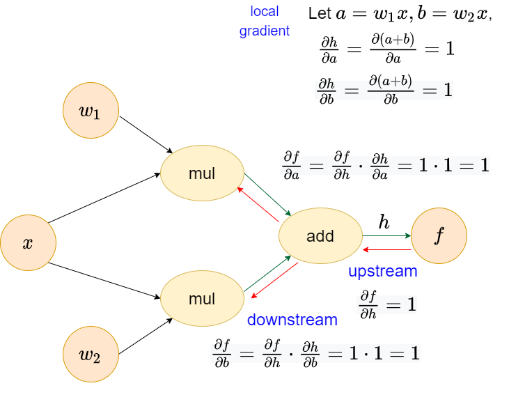
Add operator

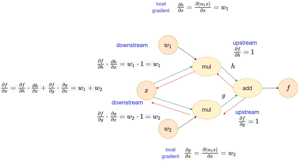
Mul operator

Validation

In the Mul operator, we have \(\frac{\partial{f}}{\partial{x}}=w_1+w_2\). Likewise, we could validate it in the numerical manner.

Let \(w_1=2, w_2=3, x=0\) and \(\epsilon=0.01\), we have \[f(0)=0\] \[f(0.01)=0.01\cdot2+0.01\cdot0.01=0.05\] \[f'(0)=\frac{0.05-0}{0.01}=5\]

In our result, we have \[\frac{\partial{f}}{\partial{x}}\Bigr|_{\substack{x=0}}=2+3=5\]

Again, they are identical which proves that the gradient is correct!

Conclusion

In this post, we take lots of time to derive the gradient by auto-differentiation and introduce the concepts called multivariate chain rule, I hope that the reader can see the beauty of autodiff and start to think about how autodiff could be implemented because we will implement it in the following series which may take some posts to illustrate the idea. Please stay tuned and we will get back!